Diffusion Models, Simply
Last night, I saw my friend drawing some anime girl while he had "Diffusion Models" opened on his laptop. And yes, that's enough motivation.
Basically, diffusion models are generative models. As in discriminative vs. generative? Right? Check out!
These models learns to reverse the gradual corruption of data by any noise, which then consists of two main parts: the Forward Process, where the original data is progressively corrupted by adding noise over time, and the Reverse Process, where the model learns to denoise the corrupted data step-by-step, eventually recovering the original data or generating new, similar data from pure noise. The model is trained to predict the noise added at each timestep, and once trained, it can generate new data by progressively denoising random noise.
Some Maths
The forward process is where we progressively add noise to the data. If we start with a clean image $( \mathbf{x}_0 )$, we apply noise at each timestep $( t )$. After several steps, the image becomes pure noise. The noise at each step is Gaussian noise, and the level of noise increases over time.
$$\mathbf{x}_t = \bar{\alpha}_t \mathbf{x}_0 + \sqrt{1 - \bar{\alpha}_t} \boldsymbol{\epsilon}$$
where, $( \mathbf{x}_0 )$ is the clean image, $( \mathbf{x}_t )$ is the noisy image at timestep ( t ) and $( \boldsymbol{\epsilon} )$ is random noise from a Gaussian distribution.
After the forward process, we want to recover the original data. This is where the reverse process comes into play. We train a neural network to learn how to predict the noise $( \boldsymbol{\epsilon} )$ that was added at each step.
$$ p_\theta(x_{t-1} \mid x_t) = \mathcal{N}(x_{t-1}; \mu_\theta(x_t, t), \sigma_t^2 I) $$
where, $\mu_\theta(x_t, t)$ is the model’s predicted mean (the denoised image at step $t-1$) and $\sigma_t^2 I$ is the variance, often a fixed schedule.
By repeatedly applying this reverse process, starting with pure noise, the model can generate new data.
The loss function used to train the model is typically the Mean Squared Error (MSE) between the model's predicted noise and the true noise added during the forward process:
$$ L = \mathbb{E} [ (\epsilon - \epsilon_\theta)^2 ] $$
where, $\epsilon$ is the true noise added to the data and $\epsilon_\theta$ is the noise predicted by the model.
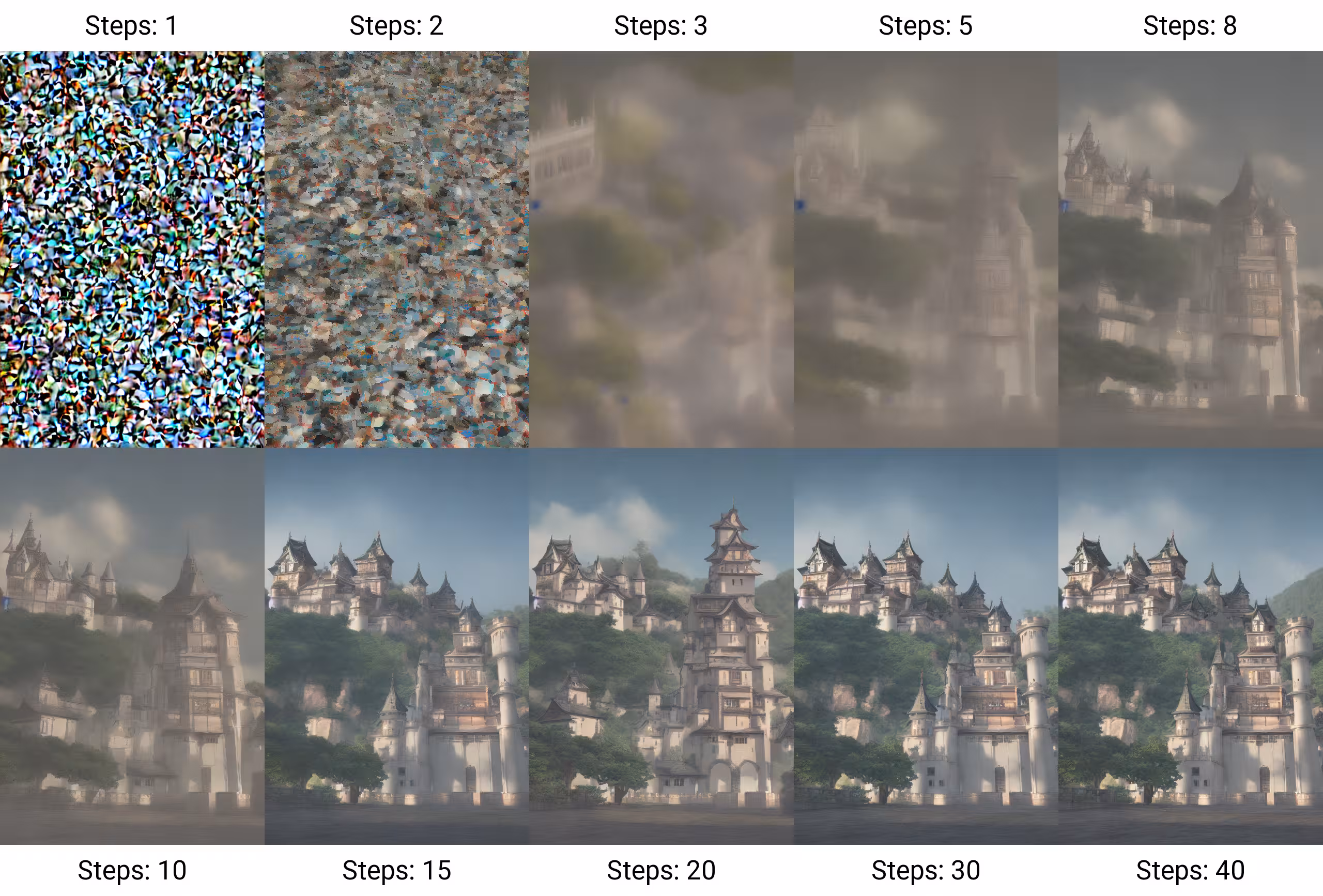
After training, the model can generate new data by starting with pure noise and applying the reverse process. The model progressively denoises the image step-by-step until it has generated a new, clean image.
Stable Diffusion is a latent diffusion model, which means it operates in a compressed latent space rather than directly on high-dimensional image space. This makes the process much faster and less computationally expensive. By using a pre-trained variational autoencoder (VAE) to compress images into latent vectors, Stable Diffusion can generate high-resolution images in just a few seconds with reasonable GPU power.
Diffusion models are known for their training stability. Unlike GANs, where the generator and discriminator need to be carefully balanced, diffusion models are less prone to mode collapse and other training instabilities.
Recent advancements have made diffusion models more computationally efficient, with models like LDM (Latent Diffusion Models) and Score-based Model using lower-resolution latent spaces, reducing memory and computation time while maintaining high-quality outputs.
But that's a discussion for another blog.
See you soon.